
The setup
A commercial PTP grandmaster of the kind you'd find in a 5G base station or on a trading floor can cost somewhere between $5,000 and $50,000. They contain temperature-compensated oscillators, hardware-timestamping Ethernet PHYs, and a certified IEEE 1588 protocol stack. They typically arrive in a 1U rackmount chassis with a datasheet promising sub-microsecond accuracy.
I made one for about $50. It is three microcontrollers on a desk, connected with a crossover Ethernet cable and a $10 GPS antenna stuck out of a window.
And it works. Not to nanosecond accuracy, let's be clear about that. But a 6-hour soak test with independent GPS-calibrated measurement shows 23 microsecond sigma (std. dev) phase alignment between the grandmaster and slave 1PPS outputs. That's roughly 1000x better than NTP, achieved on hardware you could buy with pocket change.
There's also a twist I didn't expect when I started. Along the way I detoured through a custom one-way protocol - call it LTSP (Lightweight Statistical Time Sync Protocol) - and it turned out to beat PTP on precision (4.7 µs sigma vs 23 µs) on the same hardware. PTP still has the better accuracy because it measures path delay both ways, but the precision/accuracy trade-off was the most interesting finding of the project and reshaped how I think about one-way time sync.
Bill of Materials:
| Component | Qty | Purpose | Cost ($AUD) |
|---|---|---|---|
| W5500-EVB-Pico | 2 | GM + Slave (integrates a Pico + W5500 on one board) | ~$20 |
| Raspberry Pi Pico | 1 | Independent measurement device (USB serial) | ~$4 |
| NEO-6M GPS Module | 1 | Time reference (for GM) | ~$10 |
| GPS antenna | 1 | Satellite reception | ~$10 |
| Crossover Ethernet cable | 1 | GM↔Slave link | ~$3 |
| Total | ~$47 |
Goals
I came back to sync problems to see what's now achievable on hardware that didn't exist when I last worked on this seriously. The targets for this project: a stable PTP exchange between two microcontrollers, sub-microsecond phase alignment if I could manage it, with independent measurement to keep the system honest. As a stretch goal, characterise both transports (WiFi and Ethernet) and see how close to the gold standard of sub-microsecond clock recovery I could get on ~$50 of parts.
System Architecture
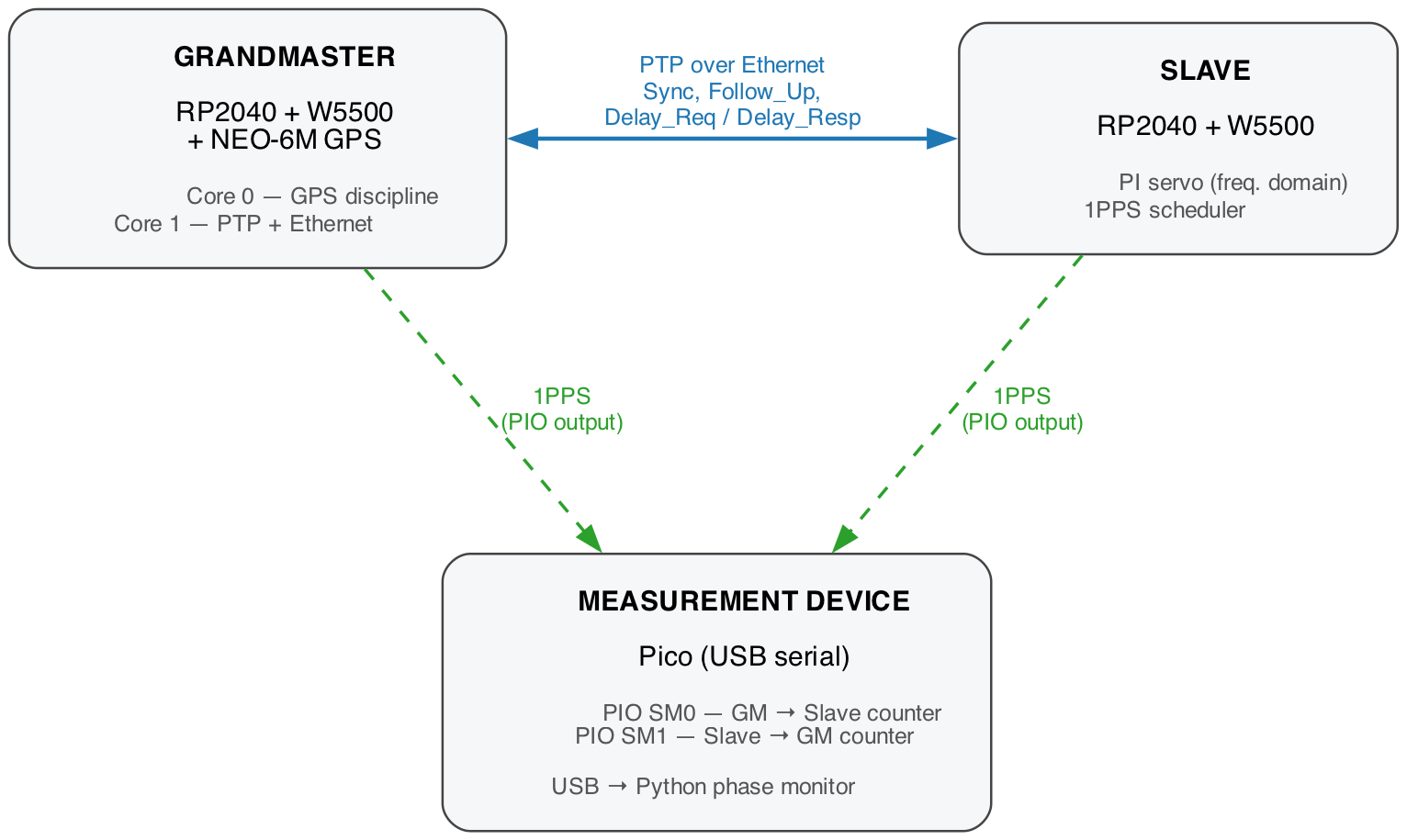
The system uses three independent devices: a grandmaster, a slave, and a measurement device. This is deliberate - the measurement device exists to keep the other two honest.
The architecture is inspired by my previous work building a frequency counter with the RP2040 and a similar GPS module.
Device 1: Grandmaster (GPS-Disciplined PTP Source)
The grandmaster is an RP2040 microcontroller paired with a W5500 SPI Ethernet module and a NEO-6M GPS receiver. It serves as the authoritative time source for the network.
The RP2040's dual-core architecture is central to the design. Core 0 handles GPS discipline exclusively - parsing NMEA sentences, capturing the GPS 1PPS rising edge with a PIO state machine, and characterizing the local crystal frequency against the GPS reference. Core 1 handles all Ethernet traffic - the W5500 SPI bus, PTP message generation (Sync + FollowUp at 1 Hz), and DelayReq/Delay_Resp processing. This separation ensures that Ethernet interrupts and SPI bus contention never interfere with the timing-critical GPS edge capture.
The grandmaster generates its own 1PPS output using a PIO-scheduled pulse, aligned to GPS time. This pulse does two things: the slave synchronises to it via PTP, and the measurement device uses it as a reference edge.
Device 2: Slave (PTP-Disciplined Clock)
The slave is a second RP2040 with a W5500 Ethernet module. It has no GPS - its only time reference comes from PTP Sync messages received over Ethernet from the grandmaster.
The slave runs a PI (proportional integral) servo in the frequency domain (the full design is covered later). When a PTP Sync/Follow_Up arrives, the slave computes its offset from the master. Rather than stepping the clock (which produces a sawtooth jitter pattern), the servo adjusts the frequency of the local clock by modifying a scale factor applied to every clock read:
// Continuous frequency correction
double scale_factor = ptp_discipline_get_scale_factor();
uint64_t ptp_elapsed_ns = (uint64_t)(elapsed_us * 1000.0 * scale_factor);
state.ptp_clock_ns += ptp_elapsed_ns;
The slave generates its own 1PPS output, scheduled by a PIO state machine that counts down to the next second boundary using the disciplined clock. If the servo is working correctly, this pulse aligns with the grandmaster's 1PPS to within tens of microseconds.
Device 3: Measurement Device (Independent Verifier)
The measurement device is a standard Raspberry Pi Pico connected to the host computer via USB serial. It takes no part in PTP or the network.
It observes the physical 1PPS outputs from the grandmaster and slave, measuring the time interval between their rising edges using two PIO state machines. One PIO program measures the GM→Slave interval (when the grandmaster pulse arrives first), and the other measures Slave→GM (when the slave pulse arrives first). Both run at 83.33 MHz (all the Picos are overclocked to 250MHz), giving 36 ns measurement resolution per tick count.
The measurement device has its own GPS module for crystal calibration, making it completely independent of both the grandmaster and slave clocks. It streams CSV-formatted phase measurements over USB serial at 1 Hz, which are then captured by processing scripts that compute statistics and store the data for later use.
This device is the "ground truth." PTP systems can report perfect synchronisation while being systematically wrong - the self-reported offset is computed from the same timestamps used for discipline, so errors can be self-consistent. The measurement device breaks this self-reference by observing the actual physical outputs.
Data Flow
The WiFi False Start
To begin with I started this work using what I had available: Raspberry Pi Pico W (WiFi) modules. The initial implementation used WiFi (on a dedicated empty network) for communication between the GM and slave devices.
Although I did get this working, the performance was terrible. WiFi's has many issues which prevent reliable PTP from working: 802.11 CSMA/CA contention windows (each transmission preceded by a variable random backoff), beacon-locked power-save wakeup, occasional re-association events, retransmits on the noisy channel, and aggregation/queueing inside the CYW43 driver. Any one of these can stall a packet by tens of milliseconds at unpredictable moments - and PTP, which assumes forward and reverse path delays are roughly symmetric and stable, simply has no answer for this. The discipline loop interprets a one-off 50 ms latency spike as a clock excursion to be corrected, then has to unwind that correction when the next packet arrives on time. The dependency on stable transport and symmetric path delay for PTP is well known, but it was useful to experience first-hand.
It was after this that I moved to Ethernet and found pre-built RP2040 modules that combine a Pico with a W5500 SPI-driven Ethernet interface.
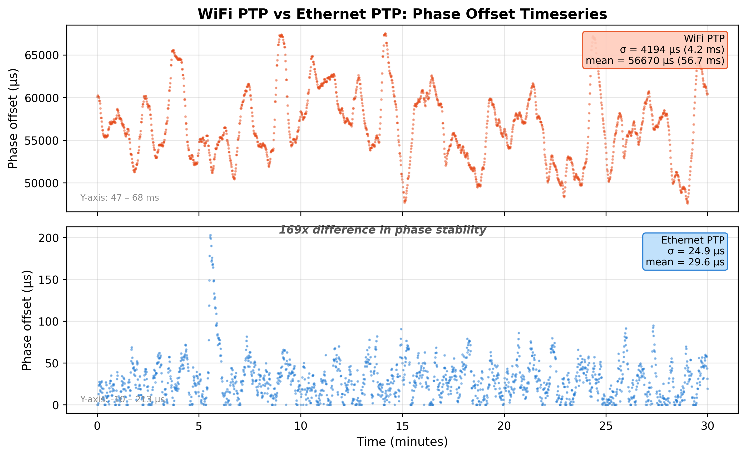
I abandoned the WiFi approach on gut instinct - the system simply wasn't tracking. Months later, with the Ethernet system stable at 23 µs and this article in mind, I went back to capture proper numbers for the WiFi case so the comparison wasn't anecdotal. I recovered the pre-Ethernet WiFi build from git history and ran the WiFi slave against the Ethernet GM with the same independent measurement process - PTP Sync/FollowUp/DelayReq/Delay_Resp over UDP/IP/WiFi.
Test methodology: 30-minute settle, 60-minute capture, 3,601 independent 1PPS phase measurements.
| Metric | WiFi PTP | Ethernet PTP |
|---|---|---|
| Phase σ | 5.95 ms | 23 µs |
| Phase mean | +58.2 ms | +27 µs |
| Path delay | 37.6 ± 13.3 ms | ~0.1 ms |
| Lock rate | 89% | 100% |
| EMA σ (5-min) | 6.4 ms | ~20 µs |
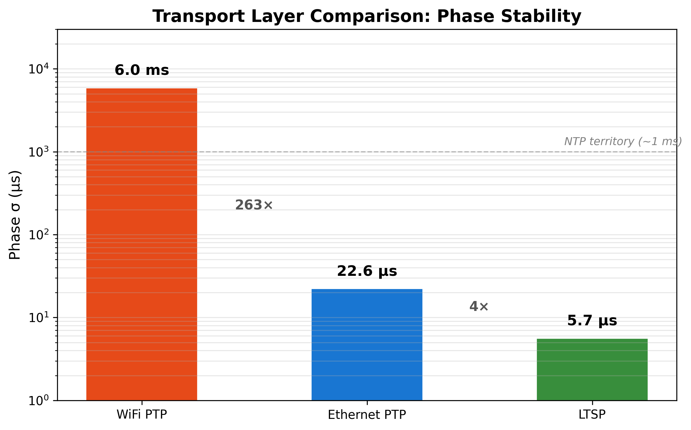
WiFi PTP is 263× worse than what we'd eventually achieve with Ethernet PTP. The path delay alone (37.6 ms mean, ±13.3 ms jitter) exceeds the Ethernet system's total phase error by three orders of magnitude. The lock rate of 89% reflects periodic unlock/relock cycles as WiFi latency spikes exceed the discipline loop's tracking bandwidth.
PIO: What Makes the RP2040 Perfect for This
Once microcontrollers become complex enough they tend to lose the deterministic characteristics which make precise timing reliable. The usual solutions are external FPGAs, dedicated timer peripherals, or simply accepting the limitation.
The RP2040 is a remarkable device with a different answer: PIO (Programmable I/O). Each RP2040 contains two PIO blocks, each with four independent state machines. These state machines run tiny assembly programs - typically 3 to 8 instructions - completely independently of the CPU, at up to the system clock rate. They are, in effect, eight small co-processors dedicated to I/O timing.
PIO is what makes this project feasible on a $4 chip. Three core building blocks were used.
The Free-Running Counter (3 instructions)
The most basic building block is a free-running countdown counter. This is the heartbeat of the timing system:
.program counter_simple
.wrap_target
    mov x, ~null            ; X = 0xFFFFFFFF
counter_loop:
    jmp x-- counter_loop [2]; Decrement, 3 cycles per iteration
.wrap
Three lines of PIO assembly. That's it. This state machine counts down from 0xFFFFFFFF at the system clock rate divided by 3, and at 250 MHz that's 83.33 MHz, or one tick every 12 nanoseconds. The CPU can read the counter value at any time without disturbing it.
Both the GM and the slave run their RP2040 at 250 MHz - twice the Pico SDK's default 125 MHz, but well within the chip's stable overclock range.
Why does this matter? The RP2040's standard time source, time_us_64(), has 1 microsecond resolution. The PIO counter gives 83× better resolution with zero CPU overhead. When you're trying to characterise crystal drift at parts-per-million levels, that factor of 83 is the difference between "can see drift" and "lost in quantisation noise."
Both the grandmaster and slave use this counter to characterise their crystal frequency against their respective references (GPS for the GM, PTP for the slave).
The 1PPS Scheduler (8 instructions)
Generating a pulse-per-second output sounds trivial - toggle a pin every second. But when to toggle it is the hard part. The pulse needs to land exactly on a second boundary as defined by the disciplined clock, and "exactly" here means within tens of nanoseconds.
.program scheduled_1pps
.wrap_target
    pull block              ; Wait for CPU to push tick count
    out x, 32               ; Load countdown into X

countdown_loop:
    jmp x-- countdown_loop  ; Count down to zero

    set pins, 1             ; Pulse HIGH
    nop [6]                 ; Hold for 8 cycles = 96ns
    set pins, 0             ; Pulse LOW
.wrap
The CPU calculates how many PIO ticks remain until the next second boundary, pushes that count into the PIO's FIFO, and the state machine autonomously counts down and fires the pulse. The pulse width is 96 nanoseconds: 8 PIO cycles at 12 ns each. This is narrow enough that the measurement device can unambiguously capture rising edges even when the two 1PPS signals are only tens of nanoseconds apart.
The critical insight: the PIO countdown is deterministic. Once the count is loaded, the pulse fires exactly N × 12ns later (actually 12ns × scale_factor later, accounting for the disciplined clock rate), with zero jitter from interrupts, cache misses, or OS scheduling. The CPU's only job is computing the count - the hard-real-time output generation happens entirely in hardware.
Edge Capture (7 instructions)
The measurement device uses a slightly different PIO program to measure the interval between two rising edges:
.program gm_to_slave_counter
.wrap_target
    wait 1 gpio 10              ; Wait for GM 1PPS rising edge
    mov x, ~null                ; X = 0xFFFFFFFF
    jmp pin done_immediately    ; If Slave already HIGH, skip

count_loop:
    jmp x-- test_slave          ; Decrement counter
test_slave:
    jmp pin slave_arrived       ; Check Slave pin
    jmp count_loop              ; Keep counting

slave_arrived:
done_immediately:
    mov y, ~x                   ; Invert: positive tick count
    mov isr, y                  ; Move to ISR
    push noblock                ; Push to FIFO
.wrap
This waits for the grandmaster's 1PPS rising edge, then counts ticks until the slave's 1PPS edge arrives. The count loop is 3 instructions per iteration, so each tick represents 36 nanoseconds (3 × 12 ns). A mirror-image program runs simultaneously on another state machine to handle the case where the slave pulse arrives first.
The measurement resolution - 36 ns - is good enough to validate a system with 23 µs of jitter by a factor of ~600×. And it costs zero CPU cycles during the counting interval. Because we are characterising the local crystal against GPS, we can use our scale_factor to be very precise about the wall time between pulses.
Why This Matters
As mentioned earlier, software timestamps on the RP2040 are limited to time_us_64(): one microsecond resolution. For a project targeting sub-25 µs accuracy, that's a 4% noise floor just from quantisation. PIO eliminates this bottleneck entirely.
More importantly, PIO provides deterministic timing. An interrupt-driven approach would add jitter from varying interrupt latency, context save/restore, and contention with other interrupts. PIO state machines run independently and identically every cycle, regardless of what the CPU is doing.
The RP2040 costs $4. The PIO programs that make this project possible total 18 lines of assembly across three programs. There is no other microcontroller in this price range that offers anything comparable for precision timing applications.
INT-Pin Pseudo Hardware Timestamping and the Asymmetry
The W5500 is a low-cost SPI Ethernet controller. It does not offer PTP-grade hardware timestamps in the protocol sense - no on-chip 1588 engine, no PHY-level capture. But it does assert an INT line when a frame is sent or received, and the RP2040 captures that INT assertion using a PIO state machine. The capture happens at PIO clock resolution (12 ns) with zero CPU jitter.
This is what I think of as pseudo hardware timestamping. It sits between two cleaner approaches: pure software timestamps (the CPU records a timestamp after the receive ISR runs, picking up microseconds of interrupt-latency jitter) and true MAC-level timestamps (a dedicated 1588 engine inside the PHY stamps each frame at the wire event - what commercial PTP gear does, at nanosecond resolution). The W5500 doesn't expose its MAC clocks, so its INT line is the best we can do - better than software, but not true HW. The INT fires after the frame has been processed inside the W5500, so there's a fixed-but-unknown delay between the wire event and the INT assertion, and that delay differs between TX and RX paths.
When I first ran the system end-to-end and compared the PTP-reported offset to the independently-measured 1PPS offset, they disagreed by about 180 µs. That's the asymmetry. Empirical measurement gave the breakdown:
| Device | TX Latency | RX Latency | Net |
|---|---|---|---|
| Slave | ~210 µs | ~135 µs | TX > RX by 75 µs |
| GM | ~265 µs | ~115 µs | TX > RX by 150 µs |
The forward path (GM TX + Slave RX) totalled ~400 µs. The reverse path (Slave TX + GM RX) totalled ~325 µs. Half the difference - 37.5 µs - is pure hardware asymmetry that PTP's symmetric-path assumption simply gets wrong.
Add the path asymmetry observed in a 53-minute crossover-cable test (96 µs) and a remaining 85 µs of unexplained systematic bias, and the total empirical correction came to +181 µs, applied as a constant to the slave's calculated offset. After this correction, the PTP-reported offset agreed with the independent measurement device to within ±1 µs.
The lesson generalises: any PTP implementation on hardware that lacks true MAC-level timestamps will have a structurally asymmetric error budget. You can characterise it and correct it on a known link, but you cannot ignore it.
The LTSP Detour
By December 2025 the basic PTP system was working at roughly 130 µs accuracy. The offset was stable, the measurement device confirmed the numbers, and the system ran without dropping pulses. It was a solid result for software-timestamped PTP on hobbyist hardware.
So naturally, I decided to try something different.
The Hypothesis
PTP's delay measurement mechanism requires a four-message exchange: Sync, FollowUp, DelayReq, DelayResp. The slave sends a DelayReq, the grandmaster timestamps its arrival and sends back a Delay_Resp. This two-way handshake is necessary to measure network path delay, but it introduces complexity - the slave needs to correlate request and response timestamps, handle out-of-order packets, and manage timeout logic.
The hypothesis was simple: on a point-to-point crossover cable with a fixed, known delay, could a one-way protocol do better by eliminating the handshake entirely and using statistical methods to characterise the link?
LTSP: Lightweight Statistical Time Sync Protocol
Over two weeks in February 2026, I designed and implemented LTSP from scratch. I sketched a draft RFC for the protocol first, working from the PTP spec and a clean-slate point-to-point cable model. The RFC has obvious shortcomings - not least being very specific to the platform I was implementing on - but it was a useful starting point.
The full RFC is in the repo: draft-user-ltsp-rp2040-04.txt.
The protocol is deliberately minimal:
- The grandmaster broadcasts a 56-byte PDU at 1 Hz. No handshake, no request/response.
- Each PDU carries the grandmaster's regression model: phase bias (a0), frequency drift (a1), model uncertainty (sigma).
- PDUs use raw Ethernet frames with EtherType
0x88B5(IEEE Local Experimental) - no IP/UDP stack needed. - The receiver runs its own linear regression over 60 samples to characterise crystal drift.
- A minimum filter tracks wire-delay estimation.
The PDU structure:
typedef struct {
    uint8_t  version;                   // Protocol version
    uint8_t  flags;                     // Status flags
    uint16_t sequence;                  // Packet sequence number
    int64_t  prev_tx_timestamp;         // TX time of previous packet
    int64_t  model_epoch;               // Reference time for model
    int64_t  source_phase_bias;         // GM phase offset (a0)
    float    source_freq_drift;         // GM frequency error in ppb (a1)
    float    model_uncertainty;         // Regression residual sigma
    int64_t  last_1pps_count;           // Most recent 1PPS edge
    uint32_t last_1pps_interval;        // Ticks between 1PPS edges
    uint32_t gm_local_processing_mean;  // Mean SPI-to-INT delay
} ltsp_pdu_t;  // 56 bytes
Instead of a PI servo, the receiver uses the regression slope directly: the frequency drift a1 maps straight to a scale factor for the local clock. No integral accumulator, no proportional gain tuning. Just set the clock rate to match the measured drift.
The regression engine itself is textbook OLS (Ordinary Least Squares) linear regression, computed fresh over a sliding window of 60 samples:
// OLS: a1 = (N*S_tau_e - S_tau*S_e) / (N*S_tau_tau - S_tau^2)
double a1 = ((double)n * S_tau_e - S_tau * S_e) / denom;
double a0 = (S_e - a1 * S_tau) / (double)n;
The complete implementation - protocol, serialisation, regression, sequence validation, minimum filter, grandmaster, receiver - came to 42 source files across 4 directories, written across fifteen commits over two weeks.
What Actually Happened
The early commits reference "-90 µs" and "-100 µs" - but that was the systematic bias, not the jitter. The bias turned out to be a fixed offset on the grandmaster's TX timestamping path. Once tracked down and corrected, LTSP's actual performance was remarkable.
The regression smoothing, combined with an adaptive IIR anchor filter (alpha decaying from 0.2 to 0.02 over 30 seconds), converged to results I frankly didn't expect from a one-way protocol:
| Run | Duration | Phase σ | Phase Mean | Peak-to-Peak |
|---|---|---|---|---|
| Feb 28 (16 min) | 16 min | 4.7 µs | +10.3 µs | 29.2 µs |
| Feb 28 (9 min) | 9 min | 5.0 µs | +10.0 µs | 24.8 µs |
| Feb 28 (46 min) | 46 min | 5.4 µs | +10.2 µs | 34.2 µs |
| Mar 2 (47 min) | 47 min | 5.7 µs | +9.7 µs | 36.5 µs |
4.7 microsecond sigma. On a one-way protocol with no handshake, using regression-based frequency discipline on a $4 microcontroller. That's nearly 5× better than the PTP system would later achieve in jitter.
How? The key is that LTSP's frequency-only discipline produces a monotonic clock. There are no discrete phase corrections: the regression slope maps directly to a clock rate, and the rate is applied continuously. This eliminates the servo-induced jitter that plagues phase-stepping approaches. The 60-sample regression window provides natural √N noise averaging, and the minimum filter handles path delay estimation.
The Limitations
LTSP's weakness is not jitter - it's accuracy. The ~+10 µs mean offset is a residual from one-way delay estimation. Without a two-way exchange, you cannot measure absolute path delay. You can estimate it statistically using a minimum filter (the shortest observed one-way delay is closest to the true propagation delay), but this estimate has an irreducible error that depends on the asymmetry of your network path.
PTP solves this with its DelayReq/DelayResp handshake: by measuring round-trip time, you can compute one-way delay as half the RTT (assuming symmetric paths). LTSP has no such mechanism, so it carries a systematic offset that requires external calibration (or acceptance).
On a crossover cable with fixed asymmetry, this is manageable. On a real network where path delays change, LTSP would drift and be largely unusable.
The Unexpected Twist
Here's the part that reshaped the project: LTSP's 4.7 µs sigma was better than PTP's eventual 23 µs. A simpler protocol, with less code, achieved tighter phase alignment.
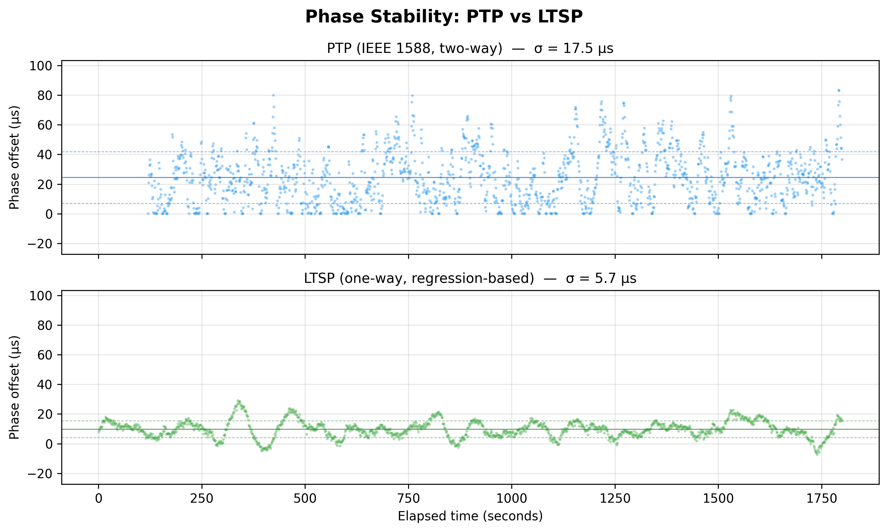
The explanation matters. LTSP's advantage comes from its frequency-only discipline - it never steps the clock, so it never introduces servo transients. PTP's two-way delay measurement gives it better absolute accuracy (the mean offset is closer to zero), but the DelayReq/DelayResp handshake adds measurement noise that the servo has to track. LTSP trades accuracy for precision.
This is the cleanest way I've found to think about one-way vs two-way time sync: two-way wins on accuracy, one-way wins on precision - and on a well-controlled link, precision is what you usually feel. The result directly informed the PTP servo redesign: the phase accumulator approach was an attempt to bring LTSP's frequency-domain smoothness to PTP's two-way accuracy. It worked - PTP sigma dropped from 130 µs to 23 µs - but LTSP's lesson is that further gains likely require reducing the servo's sensitivity to individual measurements.
Reusable Components
Beyond the performance insight, LTSP produced reusable components. The OLS regression code in ltsp_regression.c - the sliding-window linear fit that characterises frequency drift from phase samples - informed the eventual PTP phase accumulator servo design directly. The LTSP module system (ltsp_pdu.c, ltsp_sequence.c, ltsp_min_filter.c) forced clean API boundaries that improved the overall codebase quality.
Return to PTP: Applying the Learnings
In March 2026 I returned to PTP with fresh perspective from the LTSP work. The basic PTP system still worked at ~130 µs, but the LTSP experience suggested two key improvements.
Phase Accumulator Servo
The old PTP servo used a textbook PI controller in the phase domain: each PTP update computed an offset, and the servo applied a correction that adjusted the clock value. This works, but creates a characteristic sawtooth pattern in the phase error.
Here's why: between PTP updates (which arrive at 1 Hz), the local crystal runs at its natural frequency. On our RP2040, the crystal drifts at roughly +34 ppm - meaning the clock gains about 34 microseconds every second. Then the PI servo corrects this at the next update, slamming the clock back. The result is a sawtooth wave with ~34 µs peak-to-peak amplitude, regardless of how well-tuned the PI gains are.
The fix, inspired by LTSP's direct frequency-setting approach, was to move the servo to the frequency domain. Instead of correcting the clock's phase at each update, the servo adjusts the clock's rate. The RP2040 applies this rate correction continuously, on every clock read:
// Phase accumulator: servo output is frequency trim, not phase correction
static double freq_servo_update(double offset_ns, double dt_sec) {
    double p_term_ppb = PA_KP * offset_ns;   // 1µs offset → 150 ppb correction

    state.freq_trim_integral_ppb += PA_KI * offset_ns * dt_sec;

    // Anti-windup clamp at ±50 ppm
    if (state.freq_trim_integral_ppb > PA_MAX_TRIM_PPB)
        state.freq_trim_integral_ppb = PA_MAX_TRIM_PPB;
    if (state.freq_trim_integral_ppb < -PA_MAX_TRIM_PPB)
        state.freq_trim_integral_ppb = -PA_MAX_TRIM_PPB;

    return p_term_ppb + state.freq_trim_integral_ppb;
}
The servo's output - a frequency trim in parts-per-billion - feeds into the unified scale factor that the clock and 1PPS scheduler both use:
double ptp_discipline_get_scale_factor(void) {
    double crystal_ppm = state.filtered_crystal_error_ns / 1000.0;
    double total_ppb = (crystal_ppm * 1000.0) + state.freq_trim_ppb;
    double sf = 1.0 - (total_ppb / 1e9);
    cached_scale_factor = sf;
    return sf;
}
This function combines two frequency estimates: a coarse measurement from the PIO counter (characterising the crystal against PTP timestamps, typically ±34 ppm) and a fine trim from the PI servo (correcting residual error, typically ±1 ppm). The result is a single scale factor applied to every elapsed-time calculation.
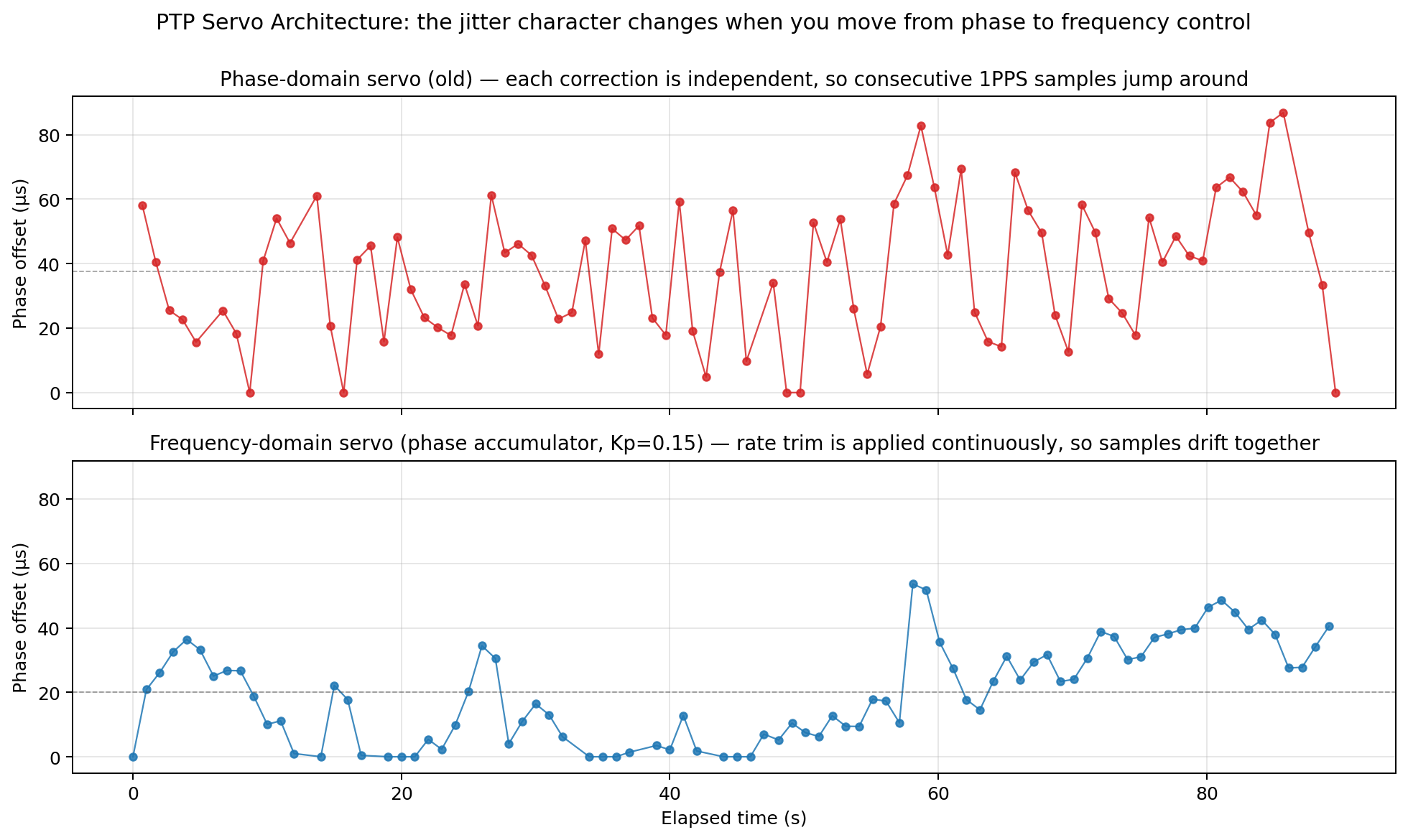
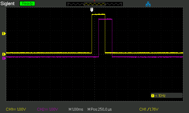
The effect was dramatic. The sawtooth in the internal clock disappeared, and the visible consequence - the jitter character of the 1PPS output - changed completely.
The chart below doesn't show a literal sawtooth wave: at 1 Hz sampling against a 1 Hz correction rate, we're aliased and the within-second drift never appears in the phase samples. But the change in jitter character is unmistakable. The old phase-stepping servo treated each correction independently, so consecutive 1PPS samples jump around within the correction envelope (top panel). The phase accumulator applies its frequency trim continuously, so consecutive samples are correlated - the clock drifts together, and the time-series shows smooth low-frequency wander instead of high-frequency hash (bottom panel).
Systematic Kp Sweep
With the phase accumulator working, the remaining question was gain tuning. The proportional gain Kp determines how aggressively the servo reacts to measured offsets - too low and it responds sluggishly, too high and it amplifies noise.
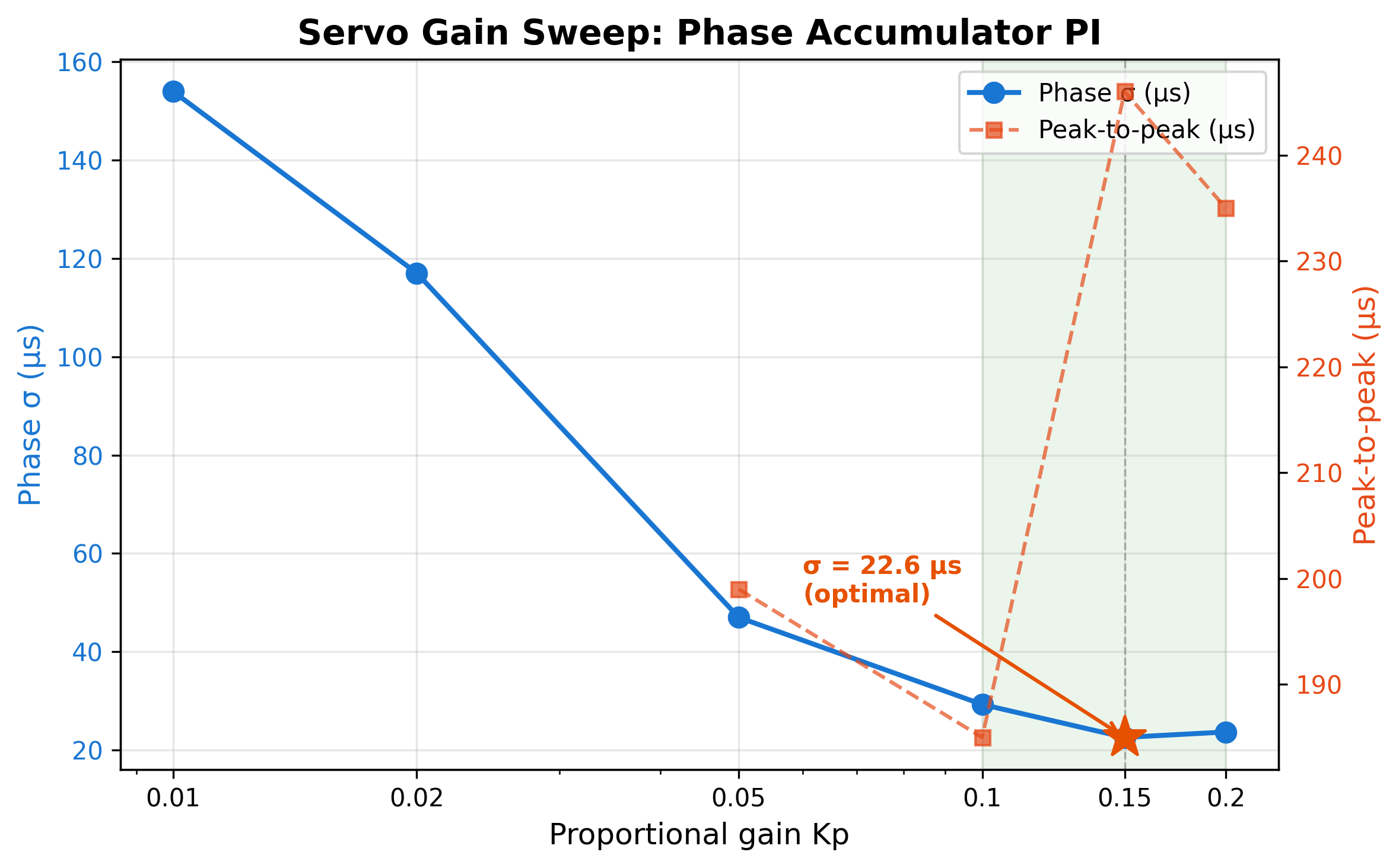
The results from a six-point sweep, each run for 60 minutes after a 30-minute settle:
| Kp | Phase σ (µs) | Peak-to-Peak (µs) | Notes |
|---|---|---|---|
| 0.01 | 154 | - | Far too conservative - can't track drift |
| 0.02 | 117 | - | Still too slow |
| 0.05 | 47 | 199 | Usable baseline |
| 0.10 | 29 | 185 | 36% improvement over baseline |
| 0.15 | 22.6 | 221 | Optimal - best sigma achieved |
| 0.20 | 23.7 | 246 | Plateau - diminishing returns, higher P-P |
The trend is clear: sigma improves monotonically from Kp=0.01 to Kp=0.15, then plateaus. Higher Kp values track offsets more aggressively but also amplify measurement noise, which shows up as increased peak-to-peak excursions. Kp=0.15 hits the sweet spot.
Something did surprise me, I had originally concluded Kp=0.05 was the peak after sweeping downward from there (0.01, 0.02 - both worse). The 0.10 → 0.15 → 0.20 sweep upward came later, and it changed the answer. Lesson worth remembering: when you sweep a parameter, sweep in both directions before locking in a result.
The 4 Hz Experiment (and Why It Failed)
With Kp optimised, the next hypothesis was obvious: faster PTP updates should give tighter control. Instead of correcting once per second, correct four times per second.
I modified the grandmaster to send Sync messages at 4 Hz and ran a test. The result was unexpected: the mean phase offset shifted by +300 µs. The sigma didn't improve meaningfully, and the entire servo operating point had moved.
The root cause: the asymmetry correction (+181 µs) had been calibrated at 1 Hz sync rate. The W5500's processing delay has a rate-dependent component - at 4 Hz the SPI bus sees more contention, the interrupt latency profile changes, and the effective asymmetry shifts. The correction that was accurate at 1 Hz became wrong at 4 Hz.
Rather than recalibrate for 4 Hz (which would require its own multi-day measurement campaign), I eliminated this variable and stayed at 1 Hz. The lesson: in timing systems, every parameter is calibrated against a specific operating point. Change the operating point and you invalidate the calibration.
The 6-Hour Soak Test
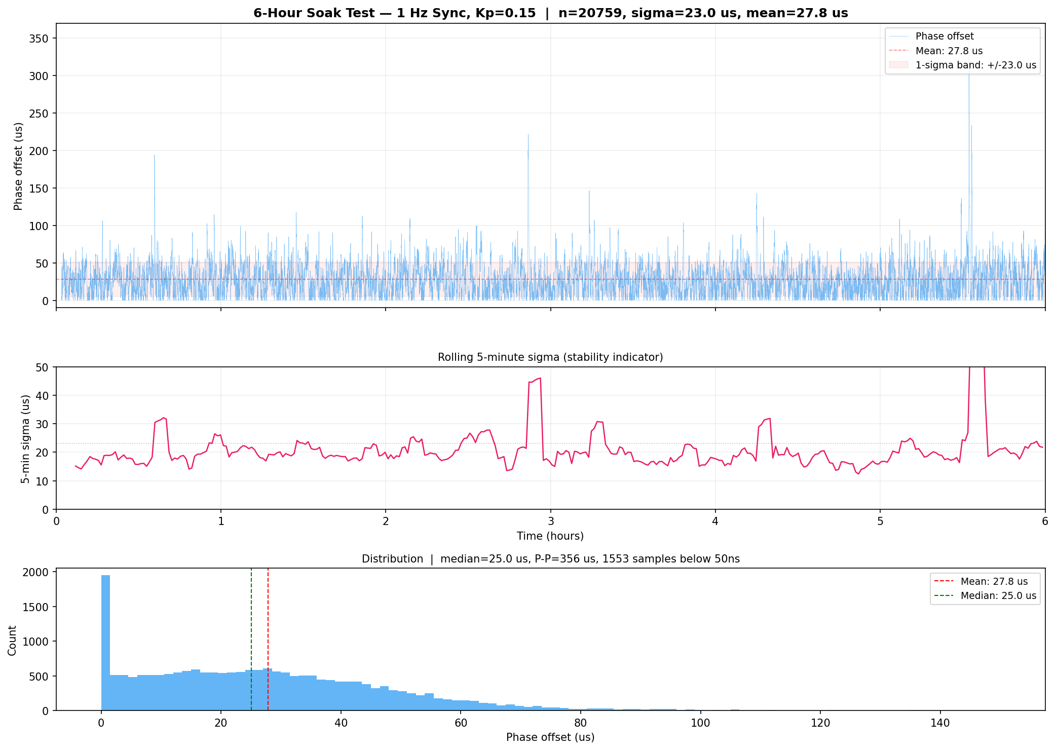
The final validation was a soak test. After 30 minutes of settling time, the system ran for 6 continuous hours with the integration test script checking phase statistics every 30 minutes.
The results held:
- Phase sigma: 23.0 µs (stable across the whole window)
- Phase mean: +27 µs (after +181 µs asymmetry correction)
- 1PPS uptime: 100% - zero dropped pulses in 21,480 seconds
- Lock maintained continuously - the servo never lost lock or required re-acquisition
This is production-quality stability on hobby hardware. The sigma didn't degrade over time, there were no thermal runaways, and the system recovered gracefully from the one W5500 FIFO stall that occurred during the test (rejected by the spike filter at the 150 µs threshold).
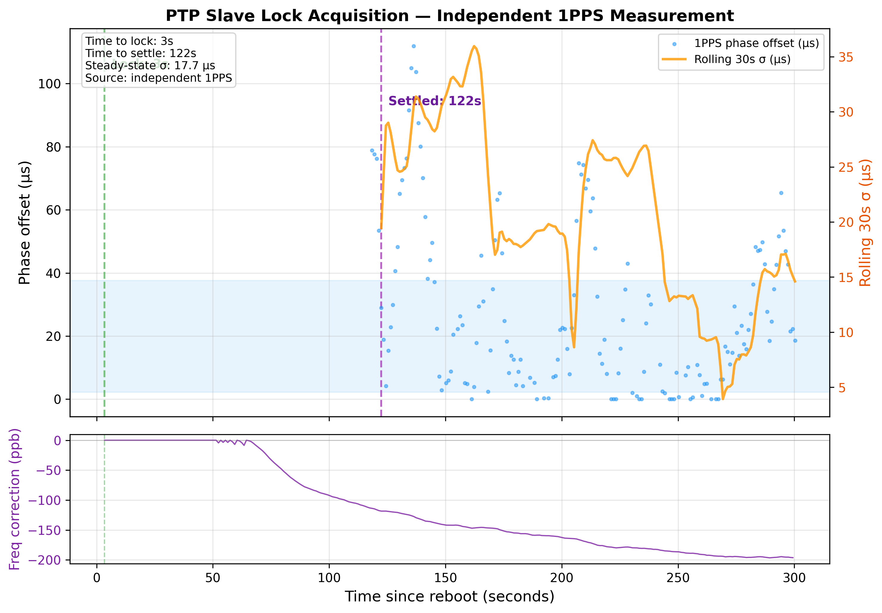
Convergence from Cold Start
A separate question: how quickly does the slave acquire lock when it boots from scratch? The convergence chart below shows that behaviour, as measured by the independent 1PPS device.
The slave's clock starts seconds off, makes repeated step corrections over the first ~60 seconds, then enters tracking mode. The measurement device can't even see both 1PPS edges until ~120 seconds in - itself a demonstration of convergence. Once in tracking mode, the rolling 30-second sigma drops below 50 µs within about 2 minutes and settles to ~18 µs steady-state.
Measurement Methodology - Keeping the System Honest
A timing system can be wrong in two distinct ways. It can be noisy - high jitter on every sample - or it can be biased, systematically off by a fixed amount that the servo will happily lock to. PTP's self-reported offset gives you a defence against neither. The slave computes its offset from the same timestamps it uses for discipline, so errors in the timestamping path produce errors in the offset that the servo then drives to zero. The system can sit in a tight-σ, happy-looking lock while the physical 1PPS pulse is hundreds of microseconds off.
This isn't theoretical. Halfway through a routine 30-minute integration test, the slave's self-reported offset spiked to −23 ms for a single sample, then recovered. Cumulative sigma for the run shot to 617 µs and the test was tagged as a FAIL. But the measurement device, watching the actual 1PPS pulses on the bench, recorded a sigma of 23.5 µs and a mean of +30 µs across the same window - solidly inside the normal operating range. The 23 ms excursion existed only in the slave's offset calculation, not in the physical output. Most likely a delayed Delay_Resp produced one bad offset value; the servo correctly ignored it (zero clock steps from that event), and the only trace was the polluted statistic.
Trusting the self-report, I'd have been chasing a phantom regression. The measurement device caught it for what it was: a calculation artefact, not a physical event. That's what the device is for.
The measurement device, in more detail
A standard Raspberry Pi Pico, no shared code with the slave or grandmaster, no participation in PTP, and its own GPS module for crystal calibration. It observes the two 1PPS lines and uses two PIO state machines to count the time between rising edges - one for each direction (GM-first and slave-first). Each tick of the counter is 3 PIO cycles at 12 ns, giving 36 ns resolution per measurement.
The output is CSV streamed over USB serial at 1 Hz: elapsed time, sequence number, phase offset in nanoseconds, which pulse arrived first, the device's own scale factor (against its own GPS), and a couple of diagnostic fields. The host-side Python - ptp_integration_test.py for harness-driven runs, ltsp_phase_serial.py for live monitoring with a braille-art terminal chart - reads the stream, computes rolling statistics, and writes the raw data to a timestamped run directory under tools/runs/.
Nothing about this can be self-consistent with the slave's errors. The measurement device's clock is GPS-disciplined separately; the counters are physical hardware reads, not derived values; the host script does its own statistics. If the slave's offset calculation goes wrong, the measurement device doesn't know and doesn't care.
Test infrastructure
The integration harness has accumulated over the four months of this project. A typical run:
ptp_integration_test.pyopens three USB serial ports - GM, slave, measurement device - and a live terminal dashboard showing rolling sigma, mean, peak-to-peak, and per-device verdicts.- The slave can be force-rebooted by USB serial number (
picotool load --ser <slave-serial>) so the grandmaster's GPS lock isn't disturbed. - The script runs for the configured duration, captures every
DISC|line from the slave, every phase sample from the measurement device, and the GM's GPS status. - At the end, it writes
summary.txtwith the headline numbers,phase.csvwith the raw measurement device data,disc.csvwith the slave's internal telemetry, and the raw serial logs.
By the time of writing there are over 95 such run directories archived in tools/runs/, each with its full raw data. The archive is part of the credibility argument - every number cited in this article can be reproduced from a CSV file in the repo. When tools/charts/sawtooth_vs_smooth.py says it loads 20260303_163948/phase.csv for the old PI servo and 20260307_102150/phase.csv for the phase accumulator, those files exist, they have the data they claim, and the chart is regenerable.
When sub-µs timing questions need a visual answer, tools/scope_waveform_phase.py interfaces with a Siglent oscilloscope over VXI-11 and pulls the full waveform rather than a screenshot - useful when the scope's display bandwidth would otherwise alias the signal.
Calibration
The one input that can't be derived from physics alone is the asymmetry correction. The slave's offset calculation assumes forward and reverse path delays are equal. They aren't, for the structural reasons covered earlier in the asymmetry section. To make the slave's self-report agree with the measurement device, I apply a constant +181 µs correction to the slave's calculated offset.
That number is empirical. It was determined by a 53-minute crossover-cable test (3,180 PTP exchanges) with the slave's offset compared sample-by-sample against the measurement device's reading. After applying the constant, the agreement is within ±1 µs.
The catch: the correction is path-specific. Change the cable, the switch, the W5500 silicon revision, or even the PTP sync rate (I saw a +300 µs operating-point shift when I tried 4 Hz syncs), and the calibration goes stale. For a fixed bench, +181 µs is honest. For deployment, you'd need to recalibrate against an external reference at the new operating point.
Validating the result
The 23 µs sigma claimed in this article is the measurement device's number, not the slave's self-report. When I say "23 µs," I mean: the rising edges of GM and slave 1PPS, observed by a separate device with its own GPS, sit within 23 µs of each other one sigma over a 6-hour soak. The slave can be off, the slave can spike, the slave can compute nonsense for one bad PTP exchange - none of that survives contact with the physical 1PPS pulse train and an independent GPS reference.
Results and Context
Here's what the system achieves after settling:
Steady-State Performance (6-Hour Soak Test):
- Phase sigma: 23 µs
- Phase mean: +27 µs (after asymmetry correction)
- 1PPS uptime: 100% (zero dropped pulses in 21,480 seconds)
- Lock acquisition: ~120 seconds to settled (<50 µs rolling sigma, independently measured)
- Spike rejection rate: < 1% (only W5500 FIFO stalls, rejected by the 150 µs spike-filter threshold)
To put these numbers in context:
| Implementation | Typical Accuracy | Hardware Cost | Key Technology |
|---|---|---|---|
| Commercial PTP (Meinberg, Microsemi) | 10–100 ns | $5K–$50K | HW timestamping PHY, OCXO |
| Software PTP on Linux/x86 (linuxptp) | 1–10 µs | $500+ | NIC HW timestamps, kernel PTP |
| This project - LTSP (one-way) | 4.7 µs | ~$50 | PIO, regression, SW timestamps |
| This project - PTP (two-way, Ethernet) | 23 µs | ~$50 | PIO, phase accum. servo |
| This project - PTP (two-way, WiFi) | 5.95 ms | ~$50 | Software timestamps, no PIO |
| NTP over internet | 1–100 ms | Free | Software only |
The WiFi result confirms what timing engineers already know: transport determinism matters more than protocol sophistication. All three project entries are on the same ~$50 hardware - only the transport layer changed. The LTSP number (4.7 µs sigma) sits comfortably in the same band as software PTP on Linux, which usually requires NIC-level hardware timestamping and runs at hundreds of times the cost.
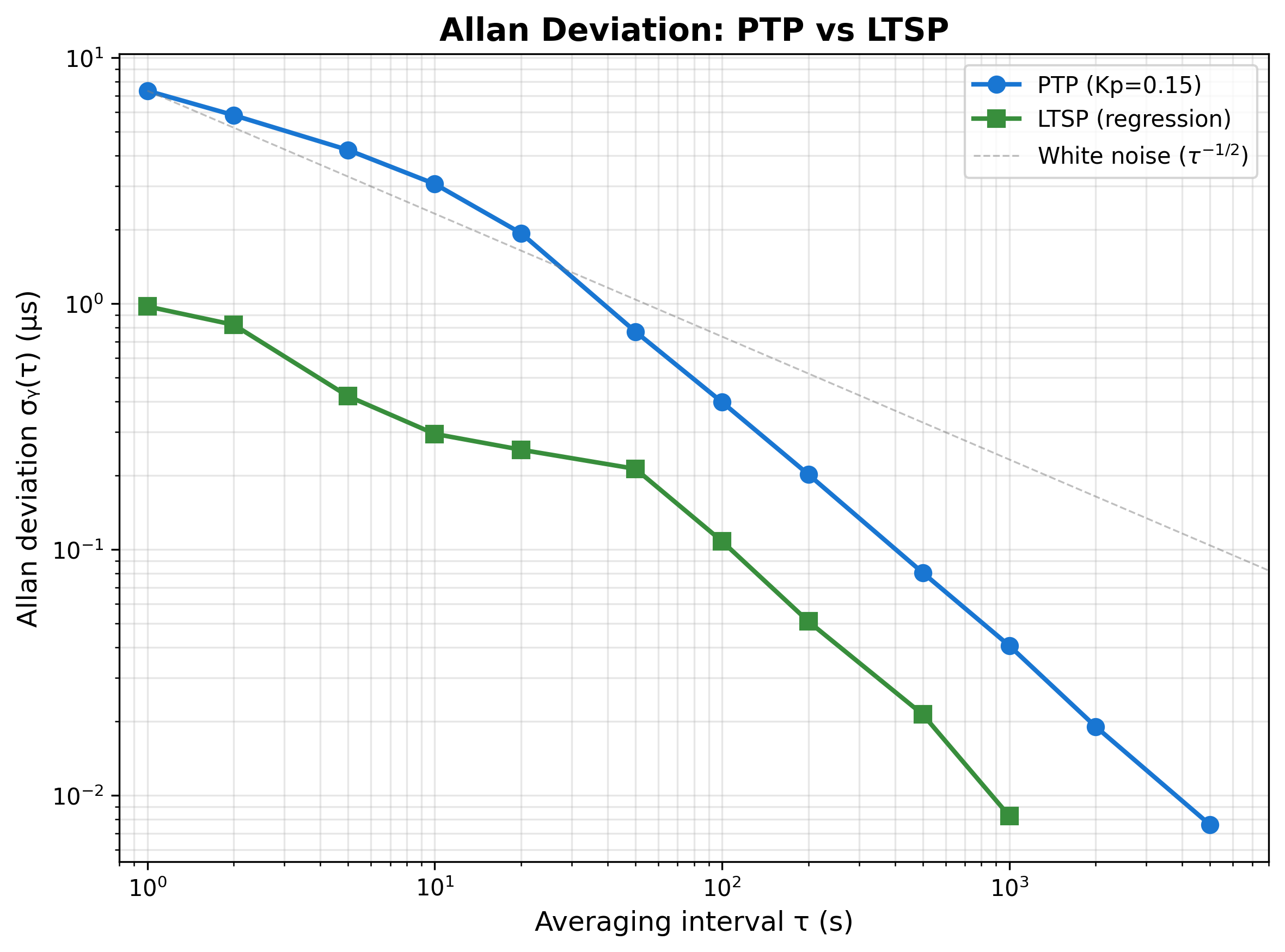
The Allan deviation plot shows both protocols follow a white-noise slope (τ^(-1/2)) at short averaging times. Essentially, if you average n samples, your error shrinks like √n - that's the signature of well-behaved random noise rather than drift or wander. LTSP starts ~7× better at τ=1s, and both converge to sub-0.01 µs stability at long averaging intervals, confirming that the underlying crystal discipline is sound - the difference at short τ is entirely servo noise.
Is 23 µs useful? To answer that it depends on your needs:
- Sensor fusion (merging data from distributed sensors): easily. Most sensor fusion algorithms assume millisecond synchronisation.
- Distributed logging (correlating events across devices): yes. 23 µs lets you establish causal ordering for any event with > 50 µs duration.
- Industrial automation (coordinated motion control): perhaps. IEC 61850 Class 1A requires ±1 µs, which we can't achieve. But simpler coordination tasks with > 100 µs deadlines would work.
- Education and research: absolutely. This is a sub-$50 platform for teaching PTP, control theory, crystal characterisation, and embedded timing.
- Audio synchronisation (AES67, Dante): perhaps. The network-layer clock sync target is in the few-µs range, which our 23 µs result is on the wrong side of; sample-accurate audio between devices typically needs tighter still, achieved via clock recovery from a PTP-disciplined network reference.
I think this system occupies a useful niche between NTP (free, millisecond-class) and professional PTP (expensive, nanosecond-class). For applications where millisecond accuracy isn't enough but microsecond accuracy isn't worth $5,000, a $50 RP2040-based system is a reasonable option.
What Limits Performance
Three factors dominate the 23 µs error budget:
- Software / pseudo-HW timestamping (~10 µs). The W5500 doesn't provide true MAC-level hardware timestamps. The RP2040 captures the INT-pin assertion via PIO, but SPI bus latency between the W5500's internal MAC processing and the INT assertion adds variable delay.
- 1 Hz update rate (~8 µs). The servo corrects once per second. Between corrections, the crystal drifts at whatever residual frequency error remains. At Kp=0.15, a 1 µs offset produces 150 ppb of correction - but the crystal's short-term Allan deviation contributes noise that the servo can't track at 1 Hz.
- Asymmetry correction residual (~5 µs). The +181 µs asymmetry correction was calibrated empirically. Any error in this calibration appears directly as a mean offset. Temperature-dependent drift in the network path delay would also show up here.
What's Next
A few threads from this project are worth pulling on.
The scale-factor hybrid. The phase accumulator already applies its frequency trim continuously, but the crystal-error component of the scale factor only refreshes when new PTP samples arrive. Closing that gap - applying the most recent crystal characterisation continuously instead of holding it constant between updates - could potentially push sigma into low single-digit µs without changing the hardware.
Hardware-timestamping PHY. The W5500's INT-line pseudo timestamps are the single largest entry in the error budget (~10 µs). Swapping the W5500 for something like a DP83640 or LAN8814 - both with real PTP engines on the PHY - would test whether the rest of the system (servo, PIO scheduling, 1PPS generation) can deliver sub-microsecond once true MAC-level timestamps are available. New driver code, but the architecture should carry over directly.
Temperature sensitivity. The crystal on the Pico is uncompensated. Indoor temperature swings of a few degrees over a day should produce a few ppm of drift; whether the servo's discipline bandwidth tracks fast enough to absorb that without sigma degradation is an open question. A 24-hour run with a temperature log alongside would answer it.
Network topology impacts. Every number in this article is from a crossover-cable benchmark - the cleanest path delay possible. Putting an unmanaged switch in the middle, or running through a multi-hop path, changes both the mean delay and the asymmetry. The +181 µs correction would need recalibration, and packet-delay variation from queueing would put a new floor on what the servo can track.
Improving LTSP. The current LTSP implementation is a research prototype: hard-coded EtherType, single-link assumption, no multicast group management or path-delay-tracking. A version suited for constrained environments - industrial sensor networks, RF-isolated subnets, anywhere you'd accept one-way trade-offs for fewer messages - would need a stricter spec, multicast handling, and a benchmark against 802.1AS on real timing-aware hardware.
Cleaning up the code. The codebase is already public but messy - it carries the full archaeology of the four-month project, including WiFi-era code, abandoned servo approaches, and experimental branches. A clean release alongside this article would help anyone trying to reproduce it: trimmed source, working CMake, the test harness, the chart-generation scripts, and a README walking through build and bench setup.
Closing
What started as a return to a problem I'd worked on nearly twenty years earlier turned into something more interesting than I expected. Microsecond time sync on ~$50 of hardware is the headline, but there are other lessons we can take away from it.
The first is the measurement device. If there is one piece of methodology I'd take from this project into any future timing work, it's this: never trust a timing system to assess itself. The slave can be wrong, the slave can be wildly wrong, and the slave can be wrong in ways that look exactly like correct behaviour. An independent measurement device - different chip, different GPS, different code, no shared timestamping path - is what gives you the right to publish a number. Everything else in this article is downstream of that.
The second is the precision–accuracy split. PTP is a two-way protocol because it has to be - without Delay_Resp it can't measure path delay - but the price of that round trip is measurement noise the servo has to track. LTSP, with no handshake, can't recover absolute path delay; but its noise floor is lower, and on a clean point-to-point link the noise floor is what you feel. Two-way wins on accuracy, one-way wins on precision. The detour through LTSP was a "failed" experiment in the strict sense - it isn't deployable as-is - but it produced the lesson that reshaped how I think about one-way time sync, and several reusable pieces that fed back into the PTP design.
The third is the RP2040 itself. Among $5 microcontrollers, the combination of dual cores, eight independent PIO state machines, and per-cycle programmable timing is genuinely unique. The 18 lines of PIO assembly that anchor this project - three for the counter, eight for the 1PPS scheduler, seven for the edge-capture - are doing work that on any other hobbyist-grade chip would require an external FPGA or a custom timer-DMA arrangement. I don't think you'd get this kind of precision out of any other $5 chip without PIO.
And the last is simply this: the work is approachable now. ~$50 in parts, four months of evenings and weekends, and a working IEEE 1588 system holding 23 µs of phase alignment over a 6-hour soak. Twenty years ago the same numbers would have required several thousand dollars and a calibrated lab. That's worth talking about I thought.
Built with RP2040, W5500, and NEO-6M GPS. Full source and test data available here.
-- Richard, May 2026